Introduction
What is Depreciation?
Depreciation is a systematic process for allocating (spreading) the cost of an asset that is used in a business to the accounting periods in which the asset is used. Depreciation is associated with buildings, equipment, vehicles, and other physical assets which will last for more than a year but will not last forever.
Reason for Depreciation
Depreciation is necessary for measuring a company’s net income in each accounting period. To demonstrate this, let’s assume that a retailer purchases a $70,000 truck on the first day of the current year, but the truck is expected to be used for seven years. It is not logical for the retailer to report the $70,000 as an expense in the current year and then report $0 expense during the remaining 6 years. However, it is logical to report $10,000 of expense in each of the 7 years that the truck is expected to be used.
Accountants often say that the purpose of depreciation is to match the cost of the truck with the revenues that are being earned by using the truck. Others say that the truck’s cost is being matched to the periods in which the truck is being used up.
Examples of Assets to be Depreciated
Some examples of assets that are depreciated include:
- Buildings (excluding land)
- Machinery and equipment
- Trucks and automobiles
- Computer systems
- Furniture and fixtures
- Land improvements (parking lots, outdoor lighting, etc.)
These assets are often described as depreciable assets, fixed assets, plant assets, productive assets, tangible assets, capital assets, and constructed assets.
How These Assets are Recorded
The assets to be depreciated are initially recorded in the accounting records at their cost. Cost is defined as all costs that were necessary to get the asset in place and ready for use.
To illustrate the cost of an asset, assume that a company paid $10,000 to purchase used equipment located 200 miles away. The company then paid $2,000 to transport the equipment to its location. Finally, the company paid $5,000 to get the equipment in working condition. The company will record the equipment in its general ledger account Equipment at the cost of $17,000.
The balance in the Equipment account will be reported on the company’s balance sheet under the asset heading property, plant and equipment.
How Depreciation is Calculated
The calculation of depreciation involves the following:
-
The asset’s cost
The asset’s cost includes all costs necessary to get the asset in place and ready for use.
-
The asset’s estimated salvage value
The asset’s estimated salvage value is the amount that the company will receive at the end of the asset’s useful life. The estimated salvage value is also referred to as the asset’s residual value or disposal value. It is common for companies to use a salvage value of $0 in the depreciation calculation.
-
The asset’s estimated useful life
The asset’s estimated useful life is the number of years (or the total units of output) that the asset is expected to be used. The useful life can be more or less than its physical life. For example, a computer may have a physical life of 10 years, but due to expected changes in software and hardware, the computer’s useful life may be 3 years.
One formula that is commonly used to calculate depreciation expense for a year is:
(Asset’s cost – estimated salvage value) / estimated years of useful life
The asset’s cost minus its estimated salvage value is known as the asset’s depreciable cost. It is the depreciable cost that is systematically allocated to expense during the asset’s useful life.
WATCH NOW
Advance Your Career with Our PRO Training
How Depreciation is Recorded
Depreciation is recorded in a company’s accounts with an adjusting entry that is typically recorded at the end of each accounting period. Except for equipment and facilities used in manufacturing, the adjusting entry for depreciation will involve the following general ledger accounts:
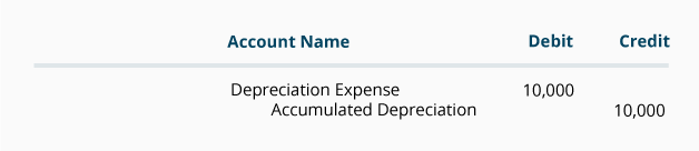
For instance, if the depreciation of a company’s delivery truck is $10,000 per year for 7 years and the company prepares only annual financial statements as of December 31, the adjusting entry for each of the 7 years will be the following:

This entry indicates that the account Depreciation Expense is being debited for $10,000 and the account Accumulated Depreciation is being credited for $10,000.
Depreciation Expense
Depreciation Expense is an income statement account. Income statement accounts are referred to as temporary accounts since their account balances are closed to a stockholders’ equity account after the annual income statement is prepared.
Since the balance is closed at the end of each accounting year, the account Depreciation Expense will begin the next accounting year with a balance of $0.
Accumulated Depreciation
Accumulated Depreciation is a balance sheet account that is associated with an asset that is being depreciated. For example, there will be an account Accumulated Depreciation – Truck that is associated with the asset account Truck.
The account Accumulated Depreciation is known as a contra asset account, since the account will appear in the asset section of the balance sheet, but it will have a credit balance (which is contrary to the normal debit balance for an asset account).
To illustrate an Accumulated Depreciation account, assume that a retailer purchased a delivery truck for $70,000 and it was recorded with a debit of $70,000 in the asset account Truck. Each year when the truck is depreciated by $10,000, the accounting entry will credit Accumulated Depreciation – Truck (instead of crediting the asset account Truck). This allows us to see both the truck’s original cost and the amount that has been depreciated since the time that the truck was put into service.
Unlike the account Depreciation Expense, the Accumulated Depreciation account is not closed at the end of each year. Instead, the balance in Accumulated Depreciation is carried forward to the next accounting period. To illustrate, let’s continue with our truck example. After the truck has been used for two years, the account Accumulated Depreciation – Truck will have a credit balance of $20,000. After three years, Accumulated Depreciation – Truck will have a credit balance of $30,000. Each year the credit balance in this account will increase by $10,000 until the credit balance reaches $70,000.
The difference between the debit balance in the asset account Truck and credit balance in Accumulated Depreciation – Truck is known as the truck’s book value or carrying value. At the end of three years the truck’s book value will be $40,000 ($70,000 minus $30,000).
Both the asset account Truck and the contra asset account Accumulated Depreciation – Truck are reported on the balance sheet under the asset heading property, plant and equipment.
Methods of Calculating Depreciation
There are many methods that a company may use to calculate the depreciation that will be reported on its financial statements. The following is a partial list of the depreciation methods that are available:
After learning some of the details in calculating depreciation using the straight-line method, we will provide examples of the following depreciation methods:
-
Units-of-activity or units-of-production
This method uses an asset’s output (instead of years) as an indicator of its useful life
-
Double-declining-balance (DDB)
This method provides more depreciation expense in the early years of the asset’s useful life and therefore less depreciation expense in the later years of the asset’s life. The calculation for the DDB method uses the asset’s book value (which is always declining) and multiplies it by two times the straight-line depreciation rate. DDB is one of the accelerated methods of depreciation.
-
Sum-of-the-years’-digits (SYD)
SYD is another accelerated method of depreciation. This means that a company will report more depreciation expense in the earlier years of the asset’s useful life and less depreciation in the later years.
The key difference in the depreciation methods involves when the asset’s cost is reported as depreciation expense on the company’s income statements:
-
If a company wants the same amount of depreciation expense each year, it will use the straight-line method.
-
If the company wants more depreciation expense in the years when an asset is used more, it will use the units-of-activity method.
-
If the company wants a greater amount of depreciation expense in the early years of an asset’s useful life (and therefore less in the later years), it will use an accelerated depreciation method such as the double-declining-balance method or the sum-of-the-years’-digits method.
Regardless of the depreciation method used, the total amount of depreciation expense over the useful life of an asset cannot exceed the asset’s depreciable cost (asset’s cost minus its estimated salvage value).
NOTE: In our explanation of depreciation, we are discussing the depreciation which is reported on a company’s financial statements. This is commonly referred to as book depreciation.
We do not discuss the depreciation that is reported on a U.S. company’s income tax return. To learn about tax depreciation, visit www.IRS.gov or discuss tax depreciation with your tax adviser. (The depreciation method used on the company’s tax return can be different from the depreciation method used on the company’s financial statements…resulting in a tax benefit.)
Straight-Line Depreciation
The most common method of depreciation used on a company’s financial statements is the straight-line method. When the straight-line method is used each full year’s depreciation expense will be the same amount.
We will illustrate the details of depreciation, and specifically the straight-line depreciation method, with the following example.
Example of Straight-Line Depreciation
A company has decided that it wants to use the straight-line method for reporting depreciation on its financial statements. The company purchased equipment for use in its business operation and provides the following information:
- On July 1, 2024, the company purchased equipment for $10,500
- The account Equipment was debited for $10,500 and the account Cash was credited for $10,500
- The company estimated that the equipment’s salvage value at the end of its useful life will be $500
- The company estimated that the equipment’s useful life will be 5 years
Given the above information, the straight-line depreciation expense for each full year that the asset is used will be $2,000 as calculated here:

If a company’s accounting year ends on December 31, the company’s income statement will report the depreciation expense as follows:

*Since the asset was acquired on July 1, 2024, only half of the annual depreciation expense amount is recorded in 2024 and 2029.
The company’s cash payment for the equipment took place on a single day in 2024 as shown here:
Since depreciation expense is reported in all years from 2024 through 2029, but the cash payment took place only at the time when the equipment was purchased, each year’s depreciation expense is often described as a noncash expense.
Recording Straight-Line Depreciation
Depreciation is recorded in the company’s accounting records through adjusting entries. Adjusting entries are recorded in the general journal using the last day of the accounting period.
Assuming the company prepares only annual financial statements for its years that end on December 31, the adjusting entries will be as follows:

If a company issues monthly financial statements, the amount of each monthly adjusting entry will be $166.67.
Visualizing the Balances in Equipment and Accumulated Depreciation
Note that the account credited in the above adjusting entries is not the asset account Equipment. Instead, the credit is entered in the contra asset account Accumulated Depreciation. The use of this contra account allows the asset account Equipment to continue to report the equipment’s cost, while also reporting in Accumulated Depreciation the total amount of depreciation expense that has been reported since the asset was acquired.
To assist in visualizing the balances in the asset account Equipment and the related contra asset account Accumulated Depreciation as of December 31, 2025 we are providing the following T-accounts:


Book Value or Carrying Value of Assets
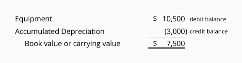
The combination of an asset account’s debit balance and its related contra asset account’s credit balance is the asset’s book value or carrying value.
Using the account balances in the T-accounts above, the book value or carrying value of the company’s equipment as of December 31, 2025 is:

When the asset’s book value is equal to the asset’s estimated salvage value, the depreciation entries will stop. If the asset continues in use, there will be $0 depreciation expense in each of the subsequent years. The asset’s cost and its accumulated depreciation balance will remain in the general ledger accounts until the asset is disposed of.
Depreciation is Based on Estimates
It is important to realize that the amount of depreciation reported by a company is an estimated amount. The reason is that the calculation of depreciation uses the following estimates:
-
Salvage value
An asset’s salvage value is also described as the asset’s disposal value, scrap value or residual value. Salvage value is an estimate of the amount the company expects to receive when it disposes of the asset at the end of the asset’s useful life. (It is common for companies to assume that an asset will have no salvage value.)
-
Useful life
The useful life of an asset is an estimate of how long the asset is expected to be used in the business. For example, a design engineer might purchase a new computer and estimate that the computer will be useful in the business for only 2 years (due to rapid advances in software and hardware). At the same time, an accountant might purchase a similar computer and estimate that it will be useful in the accounting business for 4 years. Both the design engineer’s estimated useful life of 2 years and the accountant’s estimated useful life of 4 years are correct (even though the computers are similar and may have a physical life of more than 10 years).
What Happens When an Estimated Amount Changes
For financial statements to be relevant for their users, the financial statements must be distributed soon after the accounting period ends. To achieve this requirement, accountants must estimate some amounts.
After the financial statements are distributed, it is reasonable to learn that some actual amounts are different from the estimated amounts that were included in the financial statements. Unless the differences are significant no action is required.
If there is a significant change in an asset’s estimated salvage value and/or the asset’s estimated useful life, the change in the estimate will result in a new amount of depreciation expense in the current accounting year and in the remaining years of the asset’s useful life.
NOTE: A change in the estimated salvage value or a change in the estimated useful life of an asset that is being depreciated is not considered to be an accounting error. As a result, the financial statements that have already been distributed are not changed.
A significant change in the estimated salvage value or estimated useful life will be reported in the current and remaining accounting years of the asset’s useful life.
Example of a Change in the Estimated Useful Life of an Asset
To illustrate a change in the estimated useful life of an asset, we will assume a company had the following situation:
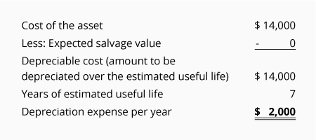
- Equipment was purchased on January 1, 2020 at a cost of $14,000
- The company originally estimated the equipment will have no salvage value
- The company originally estimated that the equipment’s useful life was 7 years
- Straight-line depreciation was used (resulting in depreciation of $2,000 in each full year)
- In 2024 the company realized that the equipment would not be useful after December 31, 2025 (instead of December 31, 2026)
- The estimated salvage value at the end of the equipment’s useful life remains at $0
- Instead of the original useful life of 7 years (January 1, 2020 through December 31, 2026), the company now estimates a total useful life of only 6 years (January 1, 2020 through December 31, 2025)
- The depreciation already reported for the years 2020 through 2023 cannot be changed since the change is not an accounting error
- The change in the estimated useful life will affect only the depreciation being reported for 2024 and 2025
Let’s first review the original straight-line depreciation using the estimates in January 2020:
The following T-accounts show that on December 31, 2023 the balance in the Equipment account is $14,000 (the cost of the equipment) and the account Accumulated Depreciation has a credit balance of $8,000:

The above accounts indicate that the book value of the equipment as of December 31, 2023 is $6,000 ($14,000 – $8,000). We also know that only two years remain (2024 and 2025) in which to depreciate the remaining $6,000 of book value. Since, the estimated salvage value is $0, the remaining $6,000 is divided by the 2 years remaining = $3,000 of depreciation expense in each of the years 2024 and 2025.
The adjusting entries for 2024 and 2025 are as follows:

As of December 31, 2025, the Accumulated Depreciation account will look like this:

Note that the depreciation amounts recorded in the years 2023 and before were not changed.
Now that you have learned the basic concepts of the depreciation reported on a company’s financial statement, we will move on to calculate depreciation using three additional depreciation methods:
- Units-of-activity (or units of production)
- Double-declining-balance
- Sum-of-the-years’-digits
Units-of-Activity Depreciation
Depreciation Not Based on Years
In most depreciation methods, an asset’s estimated useful life is expressed in years. However, in the units-of-activity method (and in the similar units-of-production method), an asset’s estimated useful life is expressed in units of output. In the units-of-activity method, the accounting period’s depreciation expense is not a function of the passage of time. Instead, each accounting period’s depreciation expense is based on the asset’s usage during the accounting period.
Examples of Units-of-Activity Depreciation
To introduce the concept of the units-of-activity method, let’s assume that a service business purchases unique equipment at a cost of $20,000. Over the equipment’s useful life, the business estimates that the equipment will produce 5,000 valuable items. Assuming there is no salvage value for the equipment, the business will report $4 ($20,000/5,000 items) of depreciation expense for each item produced. If 80 items were produced during the first month of the equipment’s use, the depreciation expense for the month will be $320 (80 items X $4). If in the next month only 10 items are produced by the equipment, only $40 (10 items X $4) of depreciation will be reported.
Now let’s illustrate the units-of-activity method of depreciation by using a different example:
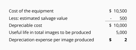
- On July 1, 2024, the company paid $10,500 to purchase special equipment to produce elaborate images for its clients
- The company estimated that this equipment will have a useful life of 5,000 images
- The company estimated that the equipment will be sold for $500 at the end of its useful life
Using the above information, the calculation of the units-of-activity method of depreciation begins with the following:

Over the life of the equipment, the maximum total amount of depreciation expense is $10,000. However, the amount of depreciation expense in any year depends on the number of images. Whether it’s a partial year or a full year is not relevant.
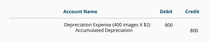
The depreciation expense for any accounting period is calculated by multiplying the number of images produced times $2 per image. For instance, if 400 images are produced from July 1 through December 31, 2024, the depreciation for 2024 will be recorded as follows:

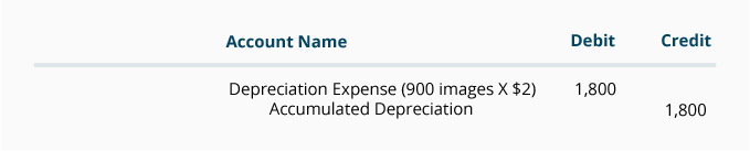
If 900 images are produced in the year 2025, the depreciation entry for 2025 will be recorded as follows:
In this example, the depreciation will continue until the credit balance in Accumulated Depreciation reaches $10,000 (the equipment’s depreciable cost). If the equipment continues to be used, no further depreciation expense will be reported. The account balances remain in the general ledger until the equipment is sold, scrapped, etc.
Double-Declining-Balance (DDB) Depreciation
DDB is an Accelerated Method of Depreciation
The double-declining-balance (DDB) method, which is also referred to as the 200%-declining-balance method, is one of the accelerated methods of depreciation. DDB is an accelerated method because more depreciation expense is reported in the early years of an asset’s life and less depreciation expense in the later years.
The “double” or “200%” means two times straight-line rate of depreciation. For instance, if an asset’s estimated useful life is 10 years, the straight-line rate of depreciation is 10% (100% divided by 10 years) per year. Therefore, the “double” or “200%” will mean a depreciation rate of 20% per year.
The “declining-balance” refers to the asset’s book value or carrying value (the asset’s cost minus its accumulated depreciation). Recall that the asset’s book value declines each time that depreciation is credited to the related contra asset account Accumulated Depreciation.
Therefore, the DDB depreciation calculation for an asset with a 10-year useful life will have a DDB depreciation rate of 20%. In the first accounting year that the asset is used, the 20% will be multiplied times the asset’s cost since there is no accumulated depreciation. In the following accounting years, the 20% is multiplied times the asset’s book value at the beginning of the accounting year. This differs from other depreciation methods where an asset’s depreciable cost is used.
In DDB depreciation the asset’s estimated salvage value is initially ignored in the calculations. However, the depreciation will stop when the asset’s book value is equal to the estimated salvage value.
NOTE: Although accelerated depreciation methods may more accurately coincide with the way some assets lose value, companies are reluctant to have their income statements show less net income and earnings per share than is required. As a result, companies are not interested in reporting larger depreciation expense in the early years of their assets’ lives (and lower depreciation in future years).
However, when it comes to taxable income and the related income tax payments, it is a different story. In the U.S. companies are permitted to use straight-line depreciation on their income statements while using accelerated depreciation on their income tax returns. You can find more information on depreciation for income tax reporting at www.IRS.gov.
Example of Double-Declining-Balance Depreciation
To illustrate the double-declining-balance method of depreciation, we will use the following information:
- A retailer purchased fixtures on January 1 at a cost of $100,000
- The estimated useful life is 10 years (resulting in a straight-line depreciation rate of 10%)
- The DDB rate will be 20% (200% or double the straight-line rate of 10%)
- The estimated salvage value at the end of its useful life is $8,000
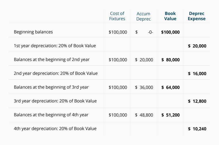
Below is a table showing the first four years of the DDB depreciation:

Note that the estimated salvage value of $8,000 was not considered in calculating each year’s depreciation expense. In our example, the depreciation expense will continue until the amount in Accumulated Depreciation reaches a credit balance of $92,000 (cost of $100,000 minus $8,000 of salvage value).
[In practice, companies often assume $0 salvage value and will switch from DDB to straight-line depreciation towards the end of the asset’s useful life in order to fully depreciate the asset’s cost.]
Sum-of-the-Years’-Digits (SYD) Depreciation
SYD is An Accelerated Method of Depreciation
The sum-of-the-years’-digits (SYD) depreciation method is also another form of accelerated depreciation since it results in more depreciation expense in the early years of the asset’s useful life and less in the later years (as compared to the straight-line method).
The “sum-of-the-years’-digits” refers to adding the digits in the years of an asset’s useful life. For example, if an asset has a useful life of 5 years, the sum of the digits 1 through 5 is equal to 15 (1 + 2 + 3 + 4 + 5).
An asset with a useful life of 10 years will have the following sum of its years’ digits:
1 + 2 + 3 + 4 + 5 + 6 + 7 + 8 + 9 + 10 = 55
A fast way to compute the sum of the digits in the asset’s useful life is to use this formula: n(n+1) divided by 2. If an asset’s useful life is 10 years, then n = 10. The sum of the digits for an asset with a useful life of 10 years = 10(10+1)/2 = 10(11)/2 = 110/2 = 55.
In the case of an asset with a 10-year useful life, the depreciation expense in the first full year of the asset’s life will be 10/55 times the asset’s depreciable cost. The depreciation for the 2nd year will be 9/55 times the asset’s depreciable cost. This pattern will continue and the depreciation for the 10th year will be 1/55 times the asset’s depreciable cost.
Example of Sum-of-the-Years’-Digits Depreciation
Now we will use the following information to calculate the SYD depreciation:
- A retailer purchased fixtures on January 1 at a cost of $115,000
- The estimated useful life is 10 years
- The estimated salvage value at the end of its useful life is $5,000
- The depreciable cost of the fixtures is $110,000 (cost of $115,000 minus the estimated salvage value of $5,000)
The depreciation amounts for the first five years of the asset’s 10-year life under SYD depreciation method are:
1st year: 10/55 times $110,000 = $20,000
2nd year: 9/55 times $110,000 = $18,000
3rd year: 8/55 times $110,000 = $16,000
4th year: 7/55 times $110,000 = $14,000
5th year: 6/55 times $110,000 = $12,000
6th year: 5/55 times $110,000 = $10,000
7th year: 4/55 times $110,000 = $8,000
8th year: 3/55 times $110,000 = $6,000
9th year: 2/55 times $110,000 = $4,000
10th year: 1/55 times $110,000 = $2,000
At the end of 10 years, the contra asset account Accumulated Depreciation will have a credit balance of $110,000. When this is combined with the debit balance of $115,000 in the asset account Fixtures, the book value of the fixtures will be $5,000 (which is equal to the estimated salvage value).
Selling a Depreciable Asset
Recording Depreciation to Date of Sale
When a depreciable asset is sold (as opposed to traded-in or exchanged for another asset), a gain or loss on the sale is likely. However, before computing the gain or loss, it is necessary to record the asset’s depreciation right up to the moment of the sale.
To amplify this step, assume that a retailer had recorded depreciation on its fleet of delivery trucks up to December 31. Three weeks later (on January 21), the company sells one of its older delivery trucks. The first step for the retailer is to record the depreciation for the three weeks that the truck was used in January.
Example of a Gain on Sale of an Asset
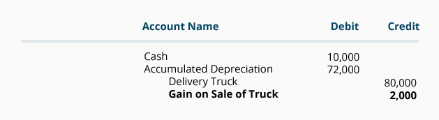
After an asset’s depreciation is recorded up to the date the asset is sold, the asset’s book value is compared to the amount received. For example, if an old delivery truck is sold and its cost was $80,000 and its accumulated depreciation at the date of the sale is $72,000, the truck’s book value at the date of the sale is $8,000.
If the retailer receives cash of $10,000 for the truck, the retailer will increase its asset cash and will remove from its assets, the truck’s book value of $8,000. Hence, the retailer has a gain of $2,000. This transaction will be recorded as follows:

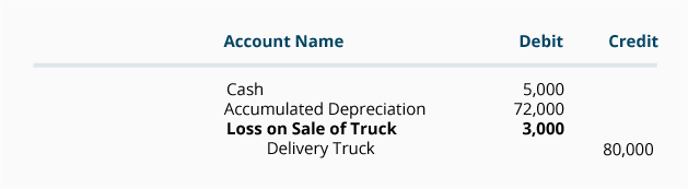
Example of a Loss on Sale of an Asset
Now let’s assume that the retailer sells the truck for $5,000 (instead of $8,000). The retailer’s cash will increase by $5,000 and its property, plant, and equipment section of the balance sheet will decrease by the book value of $8,000. As a result, the retailer will have a loss of $3,000. This transaction will be recorded as follows:
Other Information Regarding Depreciable Assets
Depreciation of Manufacturing Assets
Assuming a retailer, distributor, or service provider does not manufacture goods, the depreciation associated with its assets will be recorded and reported on its income statement as depreciation expense.
However, if a company’s depreciable assets are used in a manufacturing process, the depreciation of the manufacturing assets will not be reported directly on the income statement as depreciation expense. Instead, this depreciation will be initially recorded as part of manufacturing overhead, which is then allocated (assigned) to the goods that were manufactured.
In other words, the depreciation on the manufacturing facilities and equipment will be attached to the products manufactured. When the goods are in inventory, some of the depreciation is part of the cost of the goods reported as the asset inventory. When the goods are sold, some of the depreciation will move from the asset inventory to the cost of goods sold that is reported on the manufacturer’s income statement.
The depreciation on the non-manufacturing assets (these are assets used in the company’s selling, general and administrative activities) will be reported directly as depreciation expense on the manufacturer’s income statements.
Repairs and Maintenance Vs. Capital Expenditures
After a company’s asset has been put into service, there will likely be some future expenditures associated with the asset. If an expenditure merely maintains the asset (routine and preventative maintenance, tune ups, etc.), the expenditure is immediately reported as an expense such as Repairs and Maintenance Expense. Similarly, if a huge expenditure merely repairs a broken machine, the amount is reported as an expense such as Repairs and Maintenance Expense.
On the other hand, if an expenditure expands or improves an asset’s capabilities, the amount is not reported as an expense. Rather, the cost of the addition or improvement is recorded as an asset and should be depreciated over the remaining useful life of the asset.
The amounts spent to acquire, expand, or improve assets are referred to as capital expenditures. The amount that a company spent on capital expenditures during the accounting period is reported under investing activities on the company’s statement of cash flows.
Depreciation: Allocation Not Valuation
It is important to understand that the main purpose of depreciation is to move the cost of an asset (except the estimated salvage value) from a company’s balance sheet to depreciation expense on its income statements in a systematic manner during the asset’s useful life.
Hence, it is important to understand that depreciation is a process of allocating an asset’s cost to expense over the asset’s useful life. The purpose of depreciation is not to report the asset’s fair market value on the company’s balance sheets.
NOTE: The purpose of depreciation is to allocate an asset’s cost to expense in a systematic manner. The purpose of depreciation is not to report an asset’s current value on the company’s balance sheets.
Impairment of Assets Used in a Business
Since depreciation is not intended to report a depreciable asset’s market value, it is possible that the asset’s market value is significantly less than the asset’s book value or carrying amount. The accounting profession has addressed this situation with a mechanism to reduce the asset’s book value and to report the adjustment as an impairment loss.
There are several steps involved in determining whether an impairment loss has occurred and how to measure and report it. You can learn more about impairment losses by reading the appropriate parts of an Intermediate Accounting textbook or visiting the Financial Accounting Standards Board’s website.
Where to Go From Here
We recommend taking our Practice Quiz next, and then continuing with the rest of our Depreciation materials (see the full outline below).
We also recommend joining PRO to unlock our premium materials (certificates of achievement, video training, flashcards, visual tutorials, quick tests, quick tests with coaching, cheat sheets, guides, puzzles, business forms, printable PDF files, progress tracking, badges, points, medal rankings, activity streaks, public profile pages, and more).
Disclaimer
You should consider our materials to be an introduction to selected accounting and bookkeeping topics (with complexities likely omitted). We focus on financial statement reporting and do not discuss how that differs from income tax reporting. Therefore, you should always consult with accounting and tax professionals for assistance with your specific circumstances.

Earn Our Certificate
for This Topic
When you join PRO, you will receive instant access to 16 different Certificates of Achievement plus our Bookkeeping Certificate of Excellence.
View PRO Features